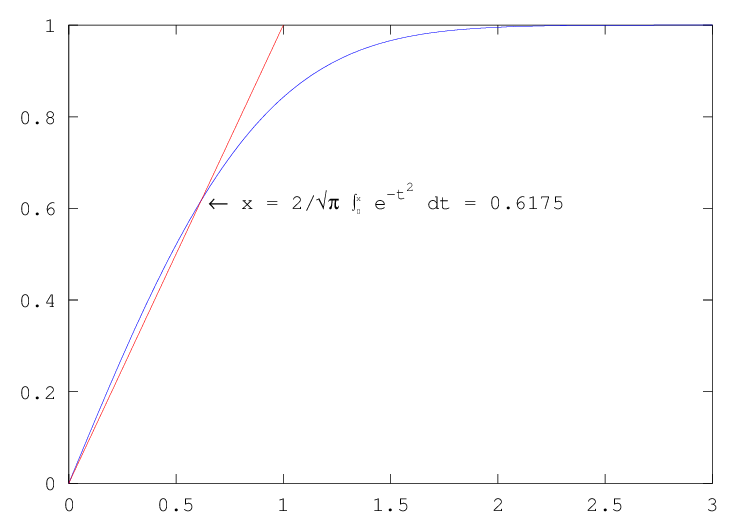
Figure 15.7: Example of inclusion of text with the TeX interpreter
You can open multiple plot windows using the figure function.
For example,
     figure (1);
     fplot (@sin, [-10, 10]);
     figure (2);
     fplot (@cos, [-10, 10]);
creates two figures, with the first displaying a sine wave and the second a cosine wave. Figure numbers must be positive integers.
Set the current plot window to plot window n. If no arguments are specified, the next available window number is chosen.
Multiple property-value pairs may be specified for the figure, but they must appear in pairs.
axis, line, and patch functions
You can create axes, line, and patch objects directly using the
axes, line, and patch functions. These objects
become children of the current axes object.
Create an axes object and return a handle to it.
Create line object from x and y and insert in current axes object. Return a handle (or vector of handles) to the line objects created.
Multiple property-value pairs may be specified for the line, but they must appear in pairs.
Create patch object from x and y with color c and insert in the current axes object. Return handle to patch object.
For a uniform colored patch, c can be given as an RGB vector, scalar value referring to the current colormap, or string value (for example, "r" or "red").
If passed a structure fv contain the fields "vertices", "faces" and optionally "facevertexcdata", create the patch based on these properties.
The optional return value h is a graphics handle to the created patch object.
See also: fill.
Create one or more filled patch objects.
The optional return value h is an array of graphics handles to the created patch objects.
See also: patch.
Plot a surface graphic object given matrices x, and y from
meshgridand a matrix z corresponding to the x and y coordinates of the surface. If x and y are vectors, then a typical vertex is (x(j), y(i), z(i,j)). Thus, columns of z correspond to different x values and rows of z correspond to different y values. If x and y are missing, they are constructed from size of the matrix z.Any additional properties passed are assigned to the surface.
The optional return value h is a graphics handle to the created surface object.
By default, Octave refreshes the plot window when a prompt is printed,
or when waiting for input. The
drawnow function is used to cause a plot window to be updated.
Update figure windows and their children. The event queue is flushed and any callbacks generated are executed. With the optional argument
"expose", only graphic objects are updated and no other events or callbacks are processed. The third calling form ofdrawnowis for debugging and is undocumented.
Only figures that are modified will be updated. The refresh
function can also be used to force an update of the current figure, even if
it is not modified.
Refresh a figure, forcing it to be redrawn. Called without an argument the current figure is redrawn, otherwise the figure pointed to by h is redrawn.
See also: drawnow.
Normally, high-level plot functions like plot or mesh call
newplot to initialize the state of the current axes so that the
next plot is drawn in a blank window with default property settings. To
have two plots superimposed over one another, use the hold
function. For example,
     hold on;
     x = -10:0.1:10;
     plot (x, sin (x));
     plot (x, cos (x));
     hold off;
displays sine and cosine waves on the same axes. If the hold state is off, consecutive plotting commands like this will only display the last plot.
Prepare graphics engine to produce a new plot. This function is called at the beginning of all high-level plotting functions. It is not normally required in user programs.
Toggle or set the 'hold' state of the plotting engine which determines whether new graphic objects are added to the plot or replace the existing objects.
hold on- Retain plot data and settings so that subsequent plot commands are displayed on a single graph.
hold all- Retain plot line color, line style, data and settings so that subsequent plot commands are displayed on a single graph with the next line color and style.
hold off- Clear plot and restore default graphics settings before each new plot command. (default).
hold- Toggle the current 'hold' state.
When given the additional argument hax, the hold state is modified only for the given axis handle.
To query the current 'hold' state use the
isholdfunction.
Return true if the next plot will be added to the current plot, or false if the plot device will be cleared before drawing the next plot.
Optionally, operate on the graphics handle h rather than the current plot.
See also: hold.
To clear the current figure, call the clf function. To clear the
current axis, call the cla function. To bring the current figure
to the top of the window stack, call the shg function. To delete
a graphics object, call delete on its index. To close the
figure window, call the close function.
Clear the current figure window.
clfoperates by deleting child graphics objects with visible handles (handlevisibility= on). If hfig is specified operate on it instead of the current figure. If the optional argument"reset"is specified, all objects including those with hidden handles are deleted.The optional return value h is the graphics handle of the figure window that was cleared.
Delete the children of the current axes with visible handles. If hax is specified and is an axes object handle, operate on it instead of the current axes. If the optional argument
"reset"is specified, also delete the children with hidden handles.See also: clf.
Delete the named file or graphics handle.
Deleting graphics objects is the proper way to remove features from a plot without clearing the entire figure.
Close figure window(s) by calling the function specified by the
"closerequestfcn"property for each figure. By default, the functionclosereqis used.See also: closereq.
Close the current figure and delete all graphics objects associated with it.
interpreter PropertyAll text objects, including titles, labels, legends, and text, include the property 'interpreter', this property determines the manner in which special control sequences in the text are rendered. If the interpreter is set to 'none', then no rendering occurs. At this point the 'latex' option is not implemented and so the 'latex' interpreter also does not interpret the text.
The 'tex' option implements a subset of TeX functionality in the rendering of the text. This allows the insertion of special characters such as Greek or mathematical symbols within the text. The special characters are also inserted with a code starting with the back-slash (\) character, as in the table tab:extended.
In addition, the formatting of the text can be changed within the string with the codes
| \bf | Bold font |
| |
| \it | Italic font |
| |
| \sl | Oblique Font |
| |
| \rm | Normal font |
|
These are be used in conjunction with the { and } characters to limit the change in the font to part of the string. For example,
xlabel ('{\bf H} = a {\bf V}')
where the character 'a' will not appear in a bold font. Note that to avoid having Octave interpret the backslash characters in the strings, the strings should be in single quotes.
It is also possible to change the fontname and size within the text
| \fontname{fontname} | Specify the font to use |
| |
| \fontsize{size} | Specify the size of the font to use |
|
Finally, the superscript and subscripting can be controlled with the '^' and '_' characters. If the '^' or '_' is followed by a { character, then all of the block surrounded by the { } pair is super- or sub-scripted. Without the { } pair, only the character immediately following the '^' or '_' is super- or sub-scripted.
| \forall | \exists | \ni |
| |
| \cong | \Delta | \Phi |
| |
| \Gamma | \vartheta | \Lambda |
| |
| \Pi | \Theta | \Sigma |
| |
| \varsigma | \Omega | \Xi |
| |
| \Psi | \perp | \alpha |
| |
| \beta | \chi | \delta |
| |
| \epsilon | \phi | \gamma |
| |
| \eta | \iota | \varphi |
| |
| \kappa | \lambda | \mu |
| |
| \nu | \o | \pi |
| |
| \theta | \rho | \sigma |
| |
| \tau | \upsilon | \varpi |
| |
| \omega | \xi | \psi |
| |
| \zeta | \sim | \Upsilon |
| |
| \prime | \leq | \infty |
| |
| \clubsuit | \diamondsuit | \heartsuit |
| |
| \spadesuit | \leftrightarrow | \leftarrow |
| |
| \uparrow | \rightarrow | \downarrow |
| |
| \circ | \pm | \geq |
| |
| \times | \propto | \partial |
| |
| \bullet | \div | \neq |
| |
| \equiv | \approx | \ldots |
| |
| \mid | \aleph | \Im |
| |
| \Re | \wp | \otimes |
| |
| \oplus | \oslash | \cap |
| |
| \cup | \supset | \supseteq |
| |
| \subset | \subseteq | \in |
| |
| \notin | \angle | \bigrightriangledown |
| |
| \langle | \rangle | \nabla |
| |
| \prod | \surd | \cdot |
| |
| \neg | \wedge | \vee |
| |
| \Leftrightarrow | \Leftarrow | \Uparrow |
| |
| \Rightarrow | \Downarrow | \diamond |
| |
| \copyright | \lfloor | \lceil |
| |
| \rfloor | \rceil | \int |
|
Table 15.1: Available special characters in TeX mode
A complete example showing the capabilities of the extended text is
     x = 0:0.01:3;
     plot(x,erf(x));
     hold on;
     plot(x,x,"r");
     axis([0, 3, 0, 1]);
     text(0.65, 0.6175, strcat('\leftarrow x = {2/\surd\pi',
     ' {\fontsize{16}\int_{\fontsize{8}0}^{\fontsize{8}x}}',
     ' e^{-t^2} dt} = 0.6175'))
The result of which can be seen in fig:extendedtext