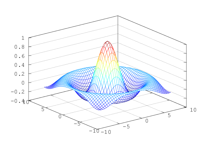
Figure 15.5: Mesh plot.
The function mesh produces mesh surface plots. For example,
     tx = ty = linspace (-8, 8, 41)';
     [xx, yy] = meshgrid (tx, ty);
     r = sqrt (xx .^ 2 + yy .^ 2) + eps;
     tz = sin (r) ./ r;
     mesh (tx, ty, tz);
produces the familiar “sombrero” plot shown in fig:mesh. Note
the use of the function meshgrid to create matrices of X and Y
coordinates to use for plotting the Z data. The ndgrid function
is similar to meshgrid, but works for N-dimensional matrices.
The meshc function is similar to mesh, but also produces a
plot of contours for the surface.
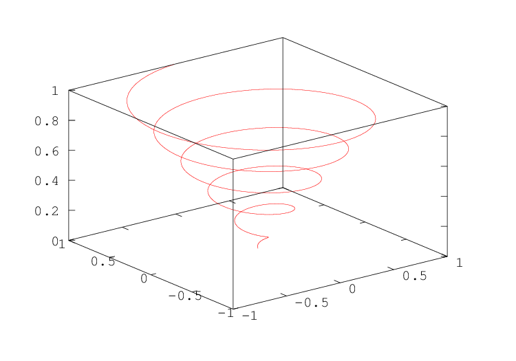
The plot3 function displays arbitrary three-dimensional data,
without requiring it to form a surface. For example,
     t = 0:0.1:10*pi;
     r = linspace (0, 1, numel (t));
     z = linspace (0, 1, numel (t));
     plot3 (r.*sin(t), r.*cos(t), z);
displays the spiral in three dimensions shown in fig:plot3.
Finally, the view function changes the viewpoint for
three-dimensional plots.
Plot a mesh given matrices x, and y from
meshgridand a matrix z corresponding to the x and y coordinates of the mesh. If x and y are vectors, then a typical vertex is (x(j), y(i), z(i,j)). Thus, columns of z correspond to different x values and rows of z correspond to different y values.The color of the mesh is derived from the
colormapand the value of z. Optionally the color of the mesh can be specified independent of z, by adding a fourth matrix, c.The optional return value h is a graphics handle to the created surface object.
Plot a mesh and contour given matrices x, and y from
meshgridand a matrix z corresponding to the x and y coordinates of the mesh. If x and y are vectors, then a typical vertex is (x(j), y(i), z(i,j)). Thus, columns of z correspond to different x values and rows of z correspond to different y values.
Plot a curtain mesh given matrices x, and y from
meshgridand a matrix z corresponding to the x and y coordinates of the mesh. If x and y are vectors, then a typical vertex is (x(j), y(i), z(i,j)). Thus, columns of z correspond to different x values and rows of z correspond to different y values.
Manipulation the mesh hidden line removal. Called with no argument the hidden line removal is toggled. The argument mode can be either 'on' or 'off' and the set of the hidden line removal is set accordingly.
Plot a surface given matrices x, and y from
meshgridand a matrix z corresponding to the x and y coordinates of the mesh. If x and y are vectors, then a typical vertex is (x(j), y(i), z(i,j)). Thus, columns of z correspond to different x values and rows of z correspond to different y values.The color of the surface is derived from the
colormapand the value of z. Optionally the color of the surface can be specified independent of z, by adding a fourth matrix, c.The optional return value h is a graphics handle to the created surface object.
Plot a surface and contour given matrices x, and y from
meshgridand a matrix z corresponding to the x and y coordinates of the mesh. If x and y are vectors, then a typical vertex is (x(j), y(i), z(i,j)). Thus, columns of z correspond to different x values and rows of z correspond to different y values.
Plot a lighted surface given matrices x, and y from
meshgridand a matrix z corresponding to the x and y coordinates of the mesh. If x and y are vectors, then a typical vertex is (x(j), y(i), z(i,j)). Thus, columns of z correspond to different x values and rows of z correspond to different y values.The light direction can be specified using L. It can be given as 2-element vector [azimuth, elevation] in degrees or as 3-element vector [lx, ly, lz]. The default value is rotated 45° counter-clockwise from the current view.
The material properties of the surface can specified using a 4-element vector P = [AM D SP exp] which defaults to p = [0.55 0.6 0.4 10].
- "AM" strength of ambient light
- "D" strength of diffuse reflection
- "SP" strength of specular reflection
- "EXP" specular exponent
The default lighting mode "cdata", changes the cdata property to give the impression of a lighted surface. Please note: the alternative "light" mode, which creates a light object to illuminate the surface is not implemented (yet).
Example:
          colormap (bone (64));
          surfl (peaks);
          shading interp;
Find the vectors normal to a meshgridded surface. The meshed gridded surface is defined by x, y, and z. If x and y are not defined, then it is assumed that they are given by
          [x, y] = meshgrid (1:size (z, 1),
                             1:size (z, 2));
If no return arguments are requested, a surface plot with the normal vectors to the surface is plotted. Otherwise the components of the normal vectors at the mesh gridded points are returned in nx, ny, and nz.
The normal vectors are calculated by taking the cross product of the diagonals of each of the quadrilaterals in the meshgrid to find the normal vectors of the centers of these quadrilaterals. The four nearest normal vectors to the meshgrid points are then averaged to obtain the normal to the surface at the meshgridded points.
An example of the use of
surfnormissurfnorm (peaks (25));
If called with one output argument and the first input argument val is a three-dimensional array that contains the data of an isosurface geometry and the second input argument iso keeps the isovalue as a scalar value then return a structure array fv that contains the fields Faces and Vertices at computed points [x, y, z] = meshgrid (1:l, 1:m, 1:n). The output argument fv can directly be taken as an input argument for the patch function.
If called with further input arguments x, y and z which are three–dimensional arrays with the same size than val then the volume data is taken at those given points.
The string input argument "noshare" is only for compatibility and has no effect. If given the string input argument "verbose" then print messages to the command line interface about the current progress.
If called with the input argument col which is a three-dimensional array of the same size than val then take those values for the interpolation of coloring the isosurface geometry. Add the field FaceVertexCData to the structure array fv.
If called with two or three output arguments then return the information about the faces f, vertices v and color data c as seperate arrays instead of a single structure array.
If called with no output argument then directly process the isosurface geometry with the patch command.
For example,
          [x, y, z] = meshgrid (1:5, 1:5, 1:5);
          val = rand (5, 5, 5);
          isosurface (x, y, z, val, .5);
will directly draw a random isosurface geometry in a graphics window. Another example for an isosurface geometry with different additional coloring
          N = 15;    # Increase number of vertices in each direction
          iso = .4;  # Change isovalue to .1 to display a sphere
          lin = linspace (0, 2, N);
          [x, y, z] = meshgrid (lin, lin, lin);
          c = abs ((x-.5).^2 + (y-.5).^2 + (z-.5).^2);
          figure (); # Open another figure window

          subplot (2,2,1); view (-38, 20);
          [f, v] = isosurface (x, y, z, c, iso);
          p = patch ("Faces", f, "Vertices", v, "EdgeColor", "none");
          set (gca, "PlotBoxAspectRatioMode", "manual", ...
                    "PlotBoxAspectRatio", [1 1 1]);
          # set (p, "FaceColor", "green", "FaceLighting", "phong");
          # light ("Position", [1 1 5]); # Available with the JHandles package

          subplot (2,2,2); view (-38, 20);
          p = patch ("Faces", f, "Vertices", v, "EdgeColor", "blue");
          set (gca, "PlotBoxAspectRatioMode", "manual", ...
                    "PlotBoxAspectRatio", [1 1 1]);
          # set (p, "FaceColor", "none", "FaceLighting", "phong");
          # light ("Position", [1 1 5]);

          subplot (2,2,3); view (-38, 20);
          [f, v, c] = isosurface (x, y, z, c, iso, y);
          p = patch ("Faces", f, "Vertices", v, "FaceVertexCData", c, ...
                     "FaceColor", "interp", "EdgeColor", "none");
          set (gca, "PlotBoxAspectRatioMode", "manual", ...
                    "PlotBoxAspectRatio", [1 1 1]);
          # set (p, "FaceLighting", "phong");
          # light ("Position", [1 1 5]);

          subplot (2,2,4); view (-38, 20);
          p = patch ("Faces", f, "Vertices", v, "FaceVertexCData", c, ...
                     "FaceColor", "interp", "EdgeColor", "blue");
          set (gca, "PlotBoxAspectRatioMode", "manual", ...
                    "PlotBoxAspectRatio", [1 1 1]);
          # set (p, "FaceLighting", "phong");
          # light ("Position", [1 1 5]);
See also: isonormals, isocolors.
If called with one output argument and the first input argument val is a three-dimensional array that contains the data for an isosurface geometry and the second input argument v keeps the vertices of an isosurface then return the normals n in form of a matrix with the same size than v at computed points [x, y, z] = meshgrid (1:l, 1:m, 1:n). The output argument n can be taken to manually set VertexNormals of a patch.
If called with further input arguments x, y and z which are three–dimensional arrays with the same size than val then the volume data is taken at those given points. Instead of the vertices data v a patch handle p can be passed to this function.
If given the string input argument "negate" as last input argument then compute the reverse vector normals of an isosurface geometry.
If no output argument is given then directly redraw the patch that is given by the patch handle p.
For example:
          function [] = isofinish (p)
            set (gca, "PlotBoxAspectRatioMode", "manual", ...
                      "PlotBoxAspectRatio", [1 1 1]);
            set (p, "VertexNormals", -get (p,"VertexNormals")); # Revert normals
            set (p, "FaceColor", "interp");
            ## set (p, "FaceLighting", "phong");
            ## light ("Position", [1 1 5]); # Available with JHandles
          endfunction

          N = 15;    # Increase number of vertices in each direction
          iso = .4;  # Change isovalue to .1 to display a sphere
          lin = linspace (0, 2, N);
          [x, y, z] = meshgrid (lin, lin, lin);
          c = abs ((x-.5).^2 + (y-.5).^2 + (z-.5).^2);
          figure (); # Open another figure window

          subplot (2,2,1); view (-38, 20);
          [f, v, cdat] = isosurface (x, y, z, c, iso, y);
          p = patch ("Faces", f, "Vertices", v, "FaceVertexCData", cdat, ...
                     "FaceColor", "interp", "EdgeColor", "none");
          isofinish (p); ## Call user function isofinish

          subplot (2,2,2); view (-38, 20);
          p = patch ("Faces", f, "Vertices", v, "FaceVertexCData", cdat, ...
                     "FaceColor", "interp", "EdgeColor", "none");
          isonormals (x, y, z, c, p); # Directly modify patch
          isofinish (p);

          subplot (2,2,3); view (-38, 20);
          p = patch ("Faces", f, "Vertices", v, "FaceVertexCData", cdat, ...
                     "FaceColor", "interp", "EdgeColor", "none");
          n = isonormals (x, y, z, c, v); # Compute normals of isosurface
          set (p, "VertexNormals", n);    # Manually set vertex normals
          isofinish (p);

          subplot (2,2,4); view (-38, 20);
          p = patch ("Faces", f, "Vertices", v, "FaceVertexCData", cdat, ...
                     "FaceColor", "interp", "EdgeColor", "none");
          isonormals (x, y, z, c, v, "negate"); # Use reverse directly
          isofinish (p);
See also: isosurface, isocolors.
If called with one output argument and the first input argument c is a three-dimensional array that contains color values and the second input argument v keeps the vertices of a geometry then return a matrix cd with color data information for the geometry at computed points [x, y, z] = meshgrid (1:l, 1:m, 1:n). The output argument cd can be taken to manually set FaceVertexCData of a patch.
If called with further input arguments x, y and z which are three–dimensional arrays of the same size than c then the color data is taken at those given points. Instead of the color data c this function can also be called with RGB values r, g, b. If input argumnets x, y, z are not given then again meshgrid computed values are taken.
Optionally, the patch handle p can be given as the last input argument to all variations of function calls instead of the vertices data v. Finally, if no output argument is given then directly change the colors of a patch that is given by the patch handle p.
For example:
          function [] = isofinish (p)
            set (gca, "PlotBoxAspectRatioMode", "manual", ...
                      "PlotBoxAspectRatio", [1 1 1]);
            set (p, "FaceColor", "interp");
            ## set (p, "FaceLighting", "flat");
            ## light ("Position", [1 1 5]); ## Available with JHandles
          endfunction

          N = 15;    # Increase number of vertices in each direction
          iso = .4;  # Change isovalue to .1 to display a sphere
          lin = linspace (0, 2, N);
          [x, y, z] = meshgrid (lin, lin, lin);
          c = abs ((x-.5).^2 + (y-.5).^2 + (z-.5).^2);
          figure (); # Open another figure window

          subplot (2,2,1); view (-38, 20);
          [f, v] = isosurface (x, y, z, c, iso);
          p = patch ("Faces", f, "Vertices", v, "EdgeColor", "none");
          cdat = rand (size (c));       # Compute random patch color data
          isocolors (x, y, z, cdat, p); # Directly set colors of patch
          isofinish (p);                # Call user function isofinish

          subplot (2,2,2); view (-38, 20);
          p = patch ("Faces", f, "Vertices", v, "EdgeColor", "none");
          [r, g, b] = meshgrid (lin, 2-lin, 2-lin);
          cdat = isocolors (x, y, z, c, v); # Compute color data vertices
          set (p, "FaceVertexCData", cdat); # Set color data manually
          isofinish (p);

          subplot (2,2,3); view (-38, 20);
          p = patch ("Faces", f, "Vertices", v, "EdgeColor", "none");
          cdat = isocolors (r, g, b, c, p); # Compute color data patch
          set (p, "FaceVertexCData", cdat); # Set color data manually
          isofinish (p);

          subplot (2,2,4); view (-38, 20);
          p = patch ("Faces", f, "Vertices", v, "EdgeColor", "none");
          r = g = b = repmat ([1:N] / N, [N, 1, N]); # Black to white
          cdat = isocolors (x, y, z, r, g, b, v);
          set (p, "FaceVertexCData", cdat);
          isofinish (p);
See also: isosurface, isonormals.
Calculate diffuse reflection strength of a surface defined by the normal vector elements sx, sy, sz. The light vector can be specified using parameter lv. It can be given as 2-element vector [azimuth, elevation] in degrees or as 3-element vector [lx, ly, lz].
Calculate specular reflection strength of a surface defined by the normal vector elements sx, sy, sz using Phong's approximation. The light and view vectors can be specified using parameter lv and vv respectively. Both can be given as 2-element vectors [azimuth, elevation] in degrees or as 3-element vector [x, y, z]. An optional 6th argument describes the specular exponent (spread) se.
Given vectors of x and y and z coordinates, and returning 3 arguments, return three-dimensional arrays corresponding to the x, y, and z coordinates of a mesh. When returning only 2 arguments, return matrices corresponding to the x and y coordinates of a mesh. The rows of xx are copies of x, and the columns of yy are copies of y. If y is omitted, then it is assumed to be the same as x, and z is assumed the same as y.
Given n vectors x1, ... xn,
ndgridreturns n arrays of dimension n. The elements of the i-th output argument contains the elements of the vector xi repeated over all dimensions different from the i-th dimension. Calling ndgrid with only one input argument x is equivalent of calling ndgrid with all n input arguments equal to x:[y1, y2, ..., yn] = ndgrid (x, ..., x)
See also: meshgrid.
Produce three-dimensional plots. Many different combinations of arguments are possible. The simplest form is
plot3 (x, y, z)in which the arguments are taken to be the vertices of the points to be plotted in three dimensions. If all arguments are vectors of the same length, then a single continuous line is drawn. If all arguments are matrices, then each column of the matrices is treated as a separate line. No attempt is made to transpose the arguments to make the number of rows match.
If only two arguments are given, as
plot3 (x, c)the real and imaginary parts of the second argument are used as the y and z coordinates, respectively.
If only one argument is given, as
plot3 (c)the real and imaginary parts of the argument are used as the y and z values, and they are plotted versus their index.
Arguments may also be given in groups of three as
plot3 (x1, y1, z1, x2, y2, z2, ...)in which each set of three arguments is treated as a separate line or set of lines in three dimensions.
To plot multiple one- or two-argument groups, separate each group with an empty format string, as
plot3 (x1, c1, "", c2, "", ...)An example of the use of
plot3isz = [0:0.05:5]; plot3 (cos (2*pi*z), sin (2*pi*z), z, ";helix;"); plot3 (z, exp (2i*pi*z), ";complex sinusoid;");
Query or set the viewpoint for the current axes. The parameters azimuth and elevation can be given as two arguments or as 2-element vector. The viewpoint can also be given with Cartesian coordinates x, y, and z. The call
view (2)sets the viewpoint to azimuth = 0 and elevation = 90, which is the default for 2-D graphs. The callview (3)sets the viewpoint to azimuth = -37.5 and elevation = 30, which is the default for 3-D graphs. If ax is given, the viewpoint is set for this axes, otherwise it is set for the current axes.
Plot slices of 3-D data/scalar fields. Each element of the 3-dimensional array v represents a scalar value at a location given by the parameters x, y, and z. The parameters x, x, and z are either 3-dimensional arrays of the same size as the array v in the "meshgrid" format or vectors. The parameters xi, etc. respect a similar format to x, etc., and they represent the points at which the array vi is interpolated using interp3. The vectors sx, sy, and sz contain points of orthogonal slices of the respective axes.
If x, y, z are omitted, they are assumed to be
x = 1:size (v, 2),y = 1:size (v, 1)andz = 1:size (v, 3).Method is one of:
- "nearest"
- Return the nearest neighbor.
- "linear"
- Linear interpolation from nearest neighbors.
- "cubic"
- Cubic interpolation from four nearest neighbors (not implemented yet).
- "spline"
- Cubic spline interpolation—smooth first and second derivatives throughout the curve.
The default method is
"linear".The optional return value h is a graphics handle to the created surface object.
Examples:
          [x, y, z] = meshgrid (linspace (-8, 8, 32));
          v = sin (sqrt (x.^2 + y.^2 + z.^2)) ./ (sqrt (x.^2 + y.^2 + z.^2));
          slice (x, y, z, v, [], 0, []);
          [xi, yi] = meshgrid (linspace (-7, 7));
          zi = xi + yi;
          slice (x, y, z, v, xi, yi, zi);
Plot a ribbon plot for the columns of y vs. x. The optional parameter width specifies the width of a single ribbon (default is 0.75). If x is omitted, a vector containing the row numbers is assumed (1:rows(Y)).
The optional return value h is a vector of graphics handles to the surface objects representing each ribbon.
Set the shading of surface or patch graphic objects. Valid arguments for type are
- "flat"
- Single colored patches with invisible edges.
- "faceted"
- Single colored patches with visible edges.
- "interp"
- Color between patch vertices are interpolated and the patch edges are invisible.
If ax is given the shading is applied to axis ax instead of the current axis.
Plot a scatter plot of the data in 3D. A marker is plotted at each point defined by the points in the vectors x, y and z. The size of the markers used is determined by s, which can be a scalar or a vector of the same length of x, y and z. If s is not given or is an empty matrix, then the default value of 8 points is used.
The color of the markers is determined by c, which can be a string defining a fixed color; a 3-element vector giving the red, green, and blue components of the color; a vector of the same length as x that gives a scaled index into the current colormap; or a n-by-3 matrix defining the colors of each of the markers individually.
The marker to use can be changed with the style argument, that is a string defining a marker in the same manner as the
plotcommand. If the argument 'filled' is given then the markers as filled. All additional arguments are passed to the underlying patch command.The optional return value h is a graphics handle to the hggroup object representing the points.
          [x, y, z] = peaks (20);
          scatter3 (x(:), y(:), z(:), [], z(:));